Friday, March 10, 2017

Dataseer Grab Challenge 2017

I recently joined the Dataseer Grab Challenge 2017, a data visualization contest to showcase local data science and design talent. The contest concluded last March 1, but I've only recently found time to sit down and write about my entry. I really enjoyed participating in this contest and wanted to share the thought process that went into it.
 
Contest Background
 
We were given around 250,000 rows of 2013 GrabTaxi data (no GrabCar). The dataset contained the following fields:
  • Source (e.g. iOS, Android, Grab booth)
  • Timestamp
  • Pick-up and drop-off location (latitude and longitude)
  • City (Metro Manila, Cebu, or Davao)
  • Fare
  • Pick-up Distance (how far the driver was upon accepting the booking)
  • State (Unallocated, i.e. no driver accepted, Completed, or Cancelled)
The instructions were open-ended: "Create a visualization of the provided dataset using a software package of your choice."
  
My Approach
 
I was initially tempted to make some kind of dashboard that shows you multiple aspects of the data at once, with interactive controls like filters and parameters to dynamically explore the data. While this is something most clients at work would ask for, I wanted to take it up a notch and used the "consulting approach" to tell a story with the data.

In the contest instructions, special emphasis was given to two metrics: Allocation Rate (AR) and Actual Allocation Rate (AAR). AR referred to the percentage of transactions that were matched with a driver, while AAR referred to the percentage of transactions that were actually completed. In other "words,"
  • AR = [# Allocated] / ([# Allocated] + [# Unallocated])
  • AAR = [# Completed] / ([# Allocated] + [# Unallocated])
      where [# Allocated] = [# Completed] + [# Cancelled]
I wanted to center my story around these metrics because they are simple to understand and are effective enough in gauging Grab's success. While digging through the data, I kept these questions in mind: Were they able to service the transactions and requests made? If not, why? How could they improve?

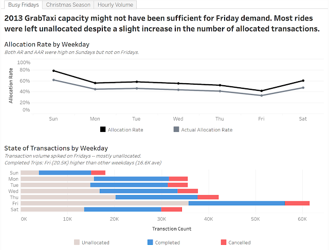
To start, I tried dissecting the data to find out which factor had a significant difference (visually, not necessarily statistically) in AR among its values. I then came up with this:


AR and AAR dipped on Fridays, but upon further inspection, this was primarily because of the sheer number of requests made. In fact, Grab was able to complete more trips on Fridays than any other weekday, but the number of unallocated transactions was just too much to handle.

How difficult is it to satisfy the unallocated demand? Allocation rate averaged just 52.6% on weekdays. Almost every other request for a taxi was not satisfied. Were taxis just at the wrong place at the wrong time?


Alright, where did all those taxis come from? How was Grab suddenly able to allocate 3,000 rides a day in December, but only 65% of the 1,200 requests on other months were allocated? Since Grab doesn't really have its own fleet (as far as I know), were more applications just approved in bulk to cater to the holiday season? If so, management can consider keeping some of that additional capacity in succeeding years to increase allocation rate in the other months.

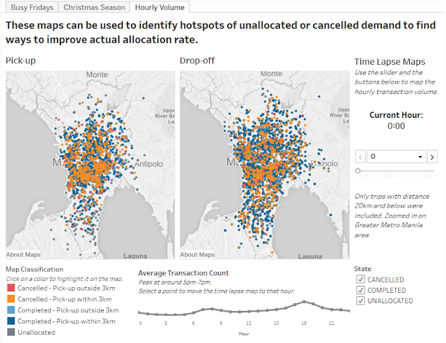
Due to the lack of fleet or capacity data, I decided to map out the pick-up and drop-off points from the dataset to see if there were any obvious patterns. As expected, there was a morning and evening peak, with the evening rush hour being the busier of the two. Most of the pick-up points were centered around the business districts, with drop-off points scattered all over the metro.

(Note: The image below is just a screenshot. Scroll to the bottom of this post for the interactive visualization.)


This was my favorite slide in the entry. I even made a video capturing the time lapse effect because the automated play function doesn't work when the visualization is uploaded to the web (Tableau Public limitation). Sorry for the awkward phone video — I had nothing else to capture it.


The colored dots may look a bit messy here, but in the interactive version, you can select a color from the legend to wash out the other colors and focus on that type of transaction. I also took some time to finalize the colors used. I initially had red, orange, yellow, and green because, admit it, a stoplight motif is commonplace in Excel files and other reports. However, it actually doesn't actually look all that great and discriminates against red-green color blindness. Good data visualizations should be color-blind friendly! Anyway, I eventually settled on these colors after testing multiple combinations, and I'd like to think that the palette blends well.

There was a snippet in the instructions about how Grab thinks that 3 km is the optimal pick-up distance — any further and the probability of cancelling exceeds a certain threshold. While I did not seek to verify that statement, the map does attempt to spot areas that were often allocated to drivers more than 3 km away. Management can then consider measures to ensure that more drivers pass by those areas.
 
Closing Thoughts
 
To be honest, I wish I spent more time on this contest. I crammed most of the work on a Sunday night and was not able to explore some dimensions of the problem nor create a rock-solid recommendation. However, I did have a lot of fun, and I am pleasantly surprised with my output. Compared to the other things I've done in this blog, this definitely looks a lot better and (I hope) is more impactful. In the end, although I didn't place in the top three, I made it to the "honorable mentions" and had my work featured on the contest page. Yay!

Here is my interactive visualization hosted on Tableau Public. If you're curious about Tableau, or if you want to do something like this but you're stuck with Excel, message me. Kape tayo. :D


After seeing the winners and other honorable mention entries, I am actually very optimistic about the future of the data visualization scene in the Philippines. Many also used "consulting style slides" like I did, and the winners definitely tackled the problem with more depth and quality visuals. Very humbling. If you're interested to see the other winning entries, check them out here:


Shoutout to Dataseer, Grab, and the AIM Analytics Club for hosting this contest. I hope to join more of these events in the future!
Monday, May 23, 2016

Job Opening - Analytics Consultant

Greetings, dear readers!

Assuming you guys exist, I would like to take a moment and plug a job opening at the company I work for. If you have taken interest to my blog and my data-driven musings, you might be interested to apply as an Analytics Consultant for Nexus Technologies.

The position is a hybrid of sorts, a cross between a management consultant and a data scientist. We are looking for people who are willing to get their hands dirty and learn as we go. We are like a startup within an established company, so expect the team to try new things, explore uncharted waters, and shoot for the moon.

That said, we are also looking for people who are passionate about analyzing data using statistical and mathematical models, building information systems for clients, and training others to become better analysts and information workers.

If you are interested, view the following job description and follow the instructions for application:
https://drive.google.com/file/d/0BzsrgvcNqkOqMUdnREFObVY1QVU/view

Help me spread the word!

Thanks,
Andrew

Friday, May 13, 2016

What Can We Learn from the Stat Wars?

A lot of friends and fellow nerds have posted their take on the controversial analysis posted by David Yap and Antonio Contreras suggesting that the VP race is tainted with electoral fraud. I think that there is already enough content to go around to challenge the validity of their claims and analysis, so I won’t go into too much detail on that (reference to those posts below). Instead, my focus will be on what we can learn about the basic principles of data analysis that are often overlooked (even by myself) when we are “in the zone” of analyzing data.
 
I can neither prove or disprove the fraud accusations. What I can do is point out other inconsistencies in the accusations and how they could have been avoided. This is especially important today, with the proliferation of data analysts or data scientists in the workplace. With more information available to us and more expectations from people who analyze data, it is critical that we are aware of the principles of data analysis to save us from making costly errors. The faulty analysis committed by Yap and Contreras can easily be the same mistakes we make ourselves when analyzing data to make business or organizational decisions.
 
DISCLAIMER: No, I am not related to David Yap. Hehe. And since we’re talking about being cautious with analysis errors, feel free to comment if you think I made a mistake as well in my analysis.
 
To non-stat friends, forgive me for the stat jargon and focus on the lessons in analysis. I think this applies to any form of critical thinking, not just in statistics or data analysis.
 

1. “Statistics means never having to say you’re certain.”


- Dr. Philip B. Stark, Professor of Statistics at University of California - Berkeley.
(Quite fittingly, Dr. Stark’s says that his research includes applications in “election auditing” among others.)
 
One of the issues I have with the analysis posted by Yap and Contreras is the way in which they call fraud, as if it is definite or there is no reasonable doubt. See here:


In statistics, we never say that we are certain about something. You have error estimates, confidence intervals, and measures of (statistical) bias. Nothing is certain, because we do not have all the data. These concepts are taught in elementary-level statistics. A true statistician knows how to report results in relation to uncertainty.
 
If we really wanted to prove electoral fraud, take a look at the electronic ballots, vote transmissions, and printed receipts instead of sample data from a partial and unofficial count. If BBM’s team can provide that kind of hard evidence, then we can approach a better conclusion about the fraud accusations.
 

2. Always validate your model.


Data analysis is not about selecting a model with the best fit (or in this case, “suspicious” R-squared values). Quoting statistician George Box, “all models are wrong, but some are useful.”
 
We use models to try to understand data, but each model comes with its own share of assumptions and prerequisites. It is our responsibility to check for model validity or “usefulness” before jumping into any conclusions. Consider the following texts:


SUMMARY: R-squared is not enough, plot the residuals.


This step is often overlooked, especially when we are trying to pull insights under time pressure. But in the end, there is no excuse for trusting an inappropriate model. 
To add to that, here’s Prof. Stark again on linear regression diagnostics: 

If the data are heteroscedastic, nonlinearly associated, or have outliers, the regression line is not a good summary of the data, and it is not appropriate to use regression to summarize the data. Heteroscedasticity, nonlinearity and outliers are easier to see in a residual plot than in a scatterplot of the raw data. There can be errors of arithmetic in calculating the regression line, so that the slope or intercept is wrong. It is easy to catch such errors by looking at residual plots, where they show up as a nonzero mean or a trend.” (heteroscedastic means that the variability of the data differs across different subsets; hetero = different, skedasis = dispersion)
 
Basically, what this means is that we should examine the plot of residuals (differences between actual values and values predicted by the model) and check for any anomalies. Ideally, there should be no patterns and outliers. We will do this graphically because it is easier to see and understand it that way.
 
Together with the standard xy-plot, I plotted the residuals of the analysis from Yap’s post and came up with this (see bottom of the post for the data and code):
Note: The data plotted here uses a subset of the entire VP Race data taken from GMA’s website. This was shared by Earl Bautista. Although this is not the exact dataset used by Yap and Contreras, I did a quick check on some data points. The numbers are the same, but Bautista’s just has more data points in between.
 
Subset is from May 9, 7:40pm (after the supposed glitch or peak of BBM’s lead) to May 10, 5:50pm. This is the period I call #LeniStrikesBack, heh.


The infamous trend line.


The linear model applied to this gives an R-squared of 0.99+, consistent with Yap’s analysis.
> summary(leniStrikesBack.lm) Call: lm(formula = BBM_Lead ~ Transmission_Rate, data = leniStrikesBack) Residuals: Min 1Q Median 3Q Max -73776 -13331 -104 16010 44524 Coefficients: Estimate Std. Error t value Pr(>|t|) (Intercept) 3741068.9 32441.9 115.3 <2e-16 *** Transmission_Rate -42798.5 382.8 -111.8 <2e-16 *** --- Signif. codes: 0 ‘***’ 0.001 ‘**’ 0.01 ‘*’ 0.05 ‘.’ 0.1 ‘ ’ 1 Residual standard error: 24680 on 51 degrees of freedom Multiple R-squared: 0.9959, Adjusted R-squared: 0.9959 F-statistic: 1.25e+04 on 1 and 51 DF, p-value: < 2.2e-16

Plotting the residuals, we get:


Curve centered at 0 with points clustered towards the right side.

If the model was an appropriate fit, the plot should show a random dispersion of points around the 0 line. Unfortunately, the plot shows a parabolic curve approximately centered at 0. No random dispersion here. 

An article on r-bloggers.com provides a guide to interpreting residual plots. See here:


Different types of residual plots and their interpretations


Ideally, our plot should be unbiased and homoscedastic (a). Unfortunately, it clearly is not. It actually falls under (f) Biased and Heteroscedastic because of its curved form and uneven dispersion (many points clustered towards the end). #bias

If Yap and Contreras did this from the start, it would have been clear that it is not appropriate to use linear regression in this case. There are other factors (non-linearity, non-randomness of samples, other relationships, etc.) affecting the two variables (% Transmission and BBM’s Lead). This should have been a warning sign for them to consider explanations such as those presented by other posters.
 
This does not remove any doubt of cheating. Again, we are never certain. It just says that the linear model is not appropriate, so other models must be considered.
 

3. Dig deeper into your data.


One of the claims made was that the trend line suggested that Leni was gaining ~40k votes per 1% of transmitted ballots. The “straightness” of the line probably further suggested that this was happening at a constant rate, making it dubious.
 
Model assumptions aside, an easy way to check this assumption is to go down one step into the data and see the rate of change of BBM’s lead over the transmission rate. This is essentially just getting the slope of the line between each data point. If the initial accusation was correct, we would expect a relatively straight line at around 40k if we plotted the slopes versus the observation numbers. Instead, we get this:


Not exactly a straight, horizontal lineat 40k.

The data is averaging close to 40k in favor of Leni, but you can argue that this looks like a parabolic, maybe even a higher-order polynomial, curve. The important point here is that it does not appear linear. This is another warning sign that the initial conclusion by Yap and Contreras is faulty and that assumptions need to be checked.
 

Putting it all together


I can summarize all 3 points by saying that any data analysis requires the analyst to always be skeptical, no matter the results. You always have to consider uncertainty and model validity when modeling, and go through your own sanity checks once you have initial conclusions. As shown by the examples above, a few extra steps to make sure these points are covered can go a long way in helping us understand the validity of our analysis.
 
Data analysis is extremely difficult because of the need to consider all these things. I have tremendous respect for anyone who is an expert in this field. But it is inevitable that we make faulty assumptions or analyses from time to time, so keep being skeptical about your conclusions. Show your work to other subject matter experts, your colleagues, or other nerdy friends. Be eager to be proven wrong! It is only in being proven wrong that we are able to progress forward with knowledge. Those who are always right (or think they are always right) never learn.
 
On the bright side, it is exciting to see the energy with which the math/stat community has approached this issue. With President-elect Duterte pushing for freedom of information, I see this as a new hope for our society. We may find ourselves with more public data to play around with, more collaboration on analysis projects, and hopefully, more informed decisions across different sectors.
 
To Mr. Yap and Mr. Contreras, and to all others involved in this, thank you for sharing your thoughts and insights. I am looking forward to a more progressive society under our newly elected leaders. Mabuhay tayong lahat!

Sources:
Data:
R Script:

Thursday, September 17, 2015

Mid-Autumn Festival Dice Game Probabilities


Ah, the familiar sight of dice rolling on a ceramic bowl.

It's the time of the year when Chinese restaurants or function rooms are filled with groups of people throwing dice into a bowl. For those who are unfamiliar with this tradition, the Chinese-Filipino community (among other overseas Chinese communities) celebrates the Mid-Autumn Festival by hosting social gatherings to play a traditional dice game. Basically, you take turns rolling the dice, and you can win prizes if your rolls match certain winning combinations.

I played my first game of the year last weekend, and I noticed that the 4th place prizes were the last ones to be consumed. This seemed to happen often in previous years, so I wanted to know if it was just coincidental or if there really was something "off" in the prize distribution probabilities.

For those who are not familiar with the game, here are the winning combinations and the corresponding number of items/prizes available per prize:


1ST PRIZE (in descending order): 1 pc


2ND PRIZE: 2 pcs
 

 3RD PRIZE: 4 pcs


4TH PRIZE: 8 pcs


5TH PRIZE: 16 pcs


6TH PRIZE: 32 pcs


To satisfy my curiosity over the events of last weekend, I computed for the theoretical probabilities of getting a particular prize in a given dice roll. For the math/stat-savvy readers, you may want to take a look at the computation logic in the appendix. I think the numbers are right, since I also ran a simulation in Excel that consistently gave roughly the same numbers. If you want, you can get the Excel file by following the link in the Appendix.

Here are my results:


One thing stands out:
The chance of getting the 4th prize is lower than the chance of getting the 3rd prize!

Okay, but does this justify why the 4th prize is usually the last to be depleted? Not quite. But from this, we can do the following (don't worry, this math isn't hard!):


As an example, if you have something that occurred 50% of the time, you can say that it occurs every other time (every 2 rolls). If you had 4 prize items to use up, and you use up 1 item every 2 rolls, it will take you about 8 rolls on average to deplete your items.

Running these equations on the probabilities presented earlier, we have:


Now, the 4th prize really stands out. On average, the 4th prize takes more than twice as long as the other prizes to be depleted. So don't roll the 4th prize too early and try to get other prizes first! There will be lots of time for you to try and get the 4th prize later on.

Other interesting take-aways from my analysis:
  • You should expect to win something for 7 out of every 10 rolls (not considering the availability of the prizes). Now you can gauge how lucky or unlucky you are at your next dice game!
  • Simulating stuff in Excel is fun!
Happy rolling! :)

---
If you want an interactive summary of everything I discussed, check out this simple dashboard! 
  

---

Appendix:

Excel File
https://www.dropbox.com/s/1pbys6u7pg4z0p7/Mid-Autumn%20Dice%20Game%20Probabilities.xlsx?dl=0


Prize Probability Calculations
Note: This section assumes that you have some background in counting principles and probability. 


1ST PRIZE


2ND PRIZE


3RD PRIZE


4TH PRIZE


5TH PRIZE


6TH PRIZE


Credits:
- Joseph Yap for the dice photo header.
- Fu character image used in the dashboard was taken from here:
http://www.ablogtowatch.com/panerai-says-fu-with-limited-edition-pam336-watch-for-china/

Sunday, July 12, 2015

Pilot: PSEI Stock Dashboard


Hello! Thanks for visiting my blog. I've been trying to setup a blog where I can follow the footsteps of data visualization gurus and jedis by making information more accessible and easy to understand. It has been a stagnant idea for a while, but I've finally gotten around to making something publish-worthy (I hope).

I have been collecting Philippine stock price data for certain stocks since mid-2014. I just take the current price (based on Bloomberg) every week for these stocks. It might sound like a lot of work, but I just take 3 minutes every weekend to do it. Not bad.

From the data I've collected, I created a simple dashboard hosted on Tableau Public. Feel free to use it to look at stocks that might interest you.

Enjoy!

P.S. Sorry about the awkward dashboard positioning and shoddy blog design. I'll fix this next time!

---

 
HOW TO INTERPRET THIS DASHBOARD

Watchlist Summary

This contains the list of stocks that I follow. You will immediately see their current price (as of the latest update), their price during the week prior to the latest update, and the % change of the stock.

Green -> the stock went up
Red -> the stock went down

Correlation Matrix

For the non-stats people: Broadly speaking, correlation is a measure (between -1 and 1) of the relationship of two sets of data. In this case, correlation measures whether Stock A moves with (positive correlation), opposite (negative correlation), or with no relation to (zero/no correlation) Stock B.

You can hover over the cells in the matrix to see the actual correlation values. The darker the color, the stronger the relationship.

Correlation can be useful when determining which stocks to invest in. You generally want to invest in stocks that are not strongly correlated to each other. For correlated stocks, when one goes up, the other is likely to go up as well. Great! But if one crashes, the other might crash with it. In short, don't put all your eggs in one basket and diversify your investments.

Time Series (Line Chart) and Other Measures

Aside from seeing how the stock moves over time, it is also to good look at the standard deviation (St. Dev) and coefficient of variance (CV). Both St. Dev and CV measure the stock price variation or how erratic the prices can be. Stocks with high variation are usually considered high risk options.

The CV is just a scaled measure of St. Dev. It is generally better to use the CV when comparing the "riskiness" of two stocks.